fit()

In the quickstart we’ve shown how to generate a 2D astrometric track (in RA cos(Dec) and Dec) and to fit a single body motion to that data.

However, this isn’t a perfect replica of the data Gaia records, nor how it is fitted.

In this section we’ll bridge that gap to give as exact an analog as possible to the gaia results and pipeline.

scanning angles

The first major difference is that Gaia (or any similar telescope) doesn’t record positions in any given co-ordinate system - instead the precession of the telescope means that each observation is along a particular axis - the scanning angle.

For bright sources Gaia measures positions both along (parallel) and across (perpendicular) to the scan direction - with the former being a much more accurate measurement than the latter (by a factor of about 3). For dim sources (G>13) only along scan measurements are recorded.

Working with angles (update: in radians!) such that 0 points towards Equatorial North and pi/2 degrees towards East we can define a set of viewing angles, or better yet use the nominal Gaia scanning-law (now with predicted observations all the way to the end of DR5! gaiascanlaw on github) to find the actual times and angles Gaia visited a patch of sky.

import astromet
import numpy as np
import matplotlib.pyplot as plt
import gaiascanlaw

ra=160
dec=-50

# scan times (decimal year) and angles (radians) for each transit in DR3
ts,phis=gaiascanlaw.scanlaw(ra,dec,tend=gaiascanlaw.times[3])

N.B. we could also use the scanning law data directly from a GOST web query, though we would need to convert the times to years (from BJD) and the angles to degrees (from radians).

which we can have a look at

ax=plt.gca()
ax.scatter(ts,phis)
ax.set_xlabel(r'observation time')
ax.set_ylabel(r'scan angle')
plt.show()

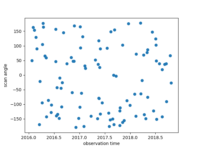
of course if we want to skip this step it’s not the end of the world to generate randomly distributed ts and phis - but as we can see there is some structure here we’d miss out on.

Let’s generate a fresh astrometric track (see the quickstart for more details)

params=astromet.params()

params.ra=ra
params.dec=dec
params.drac=0
params.ddec=0
params.pmrac=8
params.pmdec=-2
params.parallax=5

params.period=2
params.a=2
params.e=0.8
params.q=0.5
params.l=0.1

params.vphi=4.5
params.vtheta=1.5
params.vomega=5.6

params.tperi=2016

racs,decs=astromet.track(ts,params)

(this is the same system as the orange binary in quickstart)

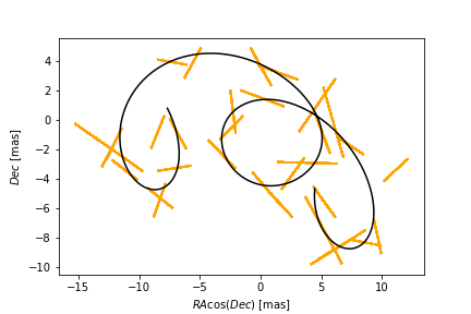
Now we want to project the true positions (racs,decs) along our scanning angle and add some random errors - let’s assume we only have along scan measurements (across scan barely contribute due to larger error anyway). If we know the magnitude we can even use appropriate Gaia-like astrometric error!

mag=18
al_error=astromet.sigma_ast(mag) # about 1.1 mas at this magnitude
errs=al_error*np.random.randn(phis.size)

obsracs=racs+errs*np.sin(phis)
obsdecs=decs+errs*np.cos(phis)

plotts=np.linspace(np.min(ts),np.max(ts),1000)
plotracs,plotdecs=astromet.track(plotts,params)

ax=plt.gca()
ax.plot([obsracs-al_error*np.sin(phis),obsracs+al_error*np.sin(phis)],
        [obsdecs-al_error*np.cos(phis),obsdecs+al_error*np.cos(phis)],c='orange')
ax.plot(plotracs,plotdecs,c='k')
ax.set_xlabel(r'$RA \cos(Dec)$ [mas]')
ax.set_ylabel(r'$Dec$ [mas]')
plt.show()

which gives the true c.o.l. track in black, and the 1D observations (with errors) in orange.

This doesn’t quite represent how Gaia actually observes these sources though - it has 9(ish) sets of CCDs which scan over the source each time it crosses the field of view - and thus it records 9 1D positions along that scan. We can simulate (and plot) these observations, including error, as such

t_obs,x_obs,phi_obs,rac_obs,dec_obs=astromet.mock_obs(ts,phis,racs,decs,err=al_error)

ax=plt.gca()
ax.scatter(t_obs,x_obs,s=10,alpha=0.5)
ax.set_xlabel(r'observation time')
ax.set_ylabel(r'$x_i = \alpha^*_i\ \sin(\phi) + \delta_i\ \cos(\phi)$')
plt.show()

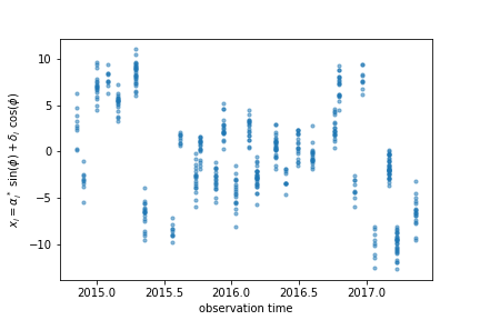
This isn’t the most illuminating plot, but this is the space Gaia actually fits in!

fitting

We’ve done all the hard work so now let’s actually fit the system

bresults=astromet.fit(t_obs,x_obs,phi_obs,al_error,ra,dec)
print(bresults)

{'vis_periods': 27, 'n_obs': 477, 'params_solved': 5, 'drac': -1.6171283773300926, 'drac_error': 0.10037615384510779, 'ddec': -1.2226831523366, 'ddec_error': 0.11038242365998072, 'drac_ddec_corr': 0.21302825773765552, 'parallax': 5.277859971259744, 'parallax_error': 0.13483844562537226, 'drac_parallax_corr': -0.052872670994359446, 'ddec_parallax_corr': 0.06289328141887433, 'pmrac': 7.623439419914979, 'pmrac_error': 0.1338069839199319, 'drac_pmrac_corr': -0.18965432423735637, 'ddec_pmrac_corr': 0.027167437980264553, 'parallax_pmrac_corr': 0.19428859515007607, 'pmdec': -2.267067734571566, 'pmdec_error': 0.1445982092420638, 'drac_pmdec_corr': 0.014967778903621016, 'ddec_pmdec_corr': -0.2395703521452692, 'parallax_pmdec_corr': -0.002380694025381034, 'pmrac_pmdec_corr': 0.20178814356775804, 'excess_noise': 0.9523963620056608, 'chi2': 871.4482146311552, 'n_good_obs': 477, 'uwe': 1.3587820245794555, 'ra_ref': 160, 'dec_ref': -50}

this gives a similar set of results to simple_fit() from the quickstart, but using a close emulation of the full Gaia astrometric pipeline AGIS <https://ui.adsabs.harvard.edu/abs/2012A%26A…538A..78L/abstract>.

In short this pipeline iteratively performs fits, inflating (if needed) an extra error term (the ‘excess_noise’) until the residuals between the observations and best fitting single-body model are consistent with this enlarged error.

We might want an exact analog to the Gaia results, so we can transform the output from fit() into the specific astrometric fields in the Gaia data model using

gaia_results=astromet.gaia_results(bresults)

or skip the middle step and jump directly from the mock data to the gaia fit:

gaia_results=astromet.gaia_fit(t_obs,x_obs,phi_obs,al_error,ra,dec)
print(gaia_results)

{'astrometric_matched_transits': 53, 'visibility_periods_used': 27, 'astrometric_n_obs_al': 477, 'astrometric_params_solved': 31, 'ra': 159.99999953448898, 'ra_error': 0.10037615384510779, 'dec': -50.00000033963421, 'dec_error': 0.11038242365998072, 'ra_dec_corr': 0.21302825773765552, 'parallax': 5.277859971259744, 'parallax_error': 0.13483844562537226, 'ra_parallax_corr': -0.052872670994359446, 'dec_parallax_corr': 0.06289328141887433, 'pmra': 7.623439419914979, 'pmra_error': 0.1338069839199319, 'ra_pmra_corr': -0.18965432423735637, 'dec_pmra_corr': 0.027167437980264553, 'parallax_pmra_corr': 0.19428859515007607, 'pmdec': -2.267067734571566, 'pmdec_error': 0.1445982092420638, 'ra_pmdec_corr': 0.014967778903621016, 'dec_pmdec_corr': -0.2395703521452692, 'parallax_pmdec_corr': -0.002380694025381034, 'pmra_pmdec_corr': 0.20178814356775804, 'astrometric_excess_noise': 0.9523963620056608, 'astrometric_chi2_al': 871.4482146311552, 'astrometric_n_good_obs_al': 477, 'uwe': 1.3587820245794555}

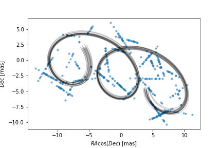
And finally we can have a look at exactly what our mock data looks like and the (range of) best fits that Gaia would find

ax=plt.gca()
for i in range(16): # plotting 16 random realizations of the fit including error
  plotts=np.linspace(np.min(ts),np.max(ts),1000)

  fit_params=astromet.params()
  fit_params.ra=bresults['ra_ref']
  fit_params.dec=bresults['dec_ref']
  fit_params.drac=bresults['drac']+np.random.randn()*bresults['drac_error']
  fit_params.ddec=bresults['ddec']+np.random.randn()*bresults['ddec_error']
  fit_params.pmrac=bresults['pmrac']+np.random.randn()*bresults['pmrac_error']
  fit_params.pmdec=bresults['pmdec']+np.random.randn()*bresults['pmdec_error']
  fit_params.parallax=bresults['parallax']+np.random.randn()*bresults['parallax_error']

  fitracs,fitdecs=astromet.track(plotts,fit_params)
  ax.plot(fitracs,fitdecs,c='k',alpha=0.2)

# plotting the actual Gaia-like observations
ax.scatter(rac_obs,dec_obs,s=10,alpha=0.5)

ax.set_xlabel(r'$RA \cos(Dec)$ [mas]')
ax.set_ylabel(r'$Dec$ [mas]')
plt.show()